Learn the Basics
This chapter introduces you to the basic conception of optical flow, and the framework of MMFlow, and provides links to detailed tutorials about MMFlow.
What is Optical flow estimation
Optical flow is a 2D velocity field, representing the apparent 2D image motion of pixels from the reference image to the target image [1]. The task can be defined as follows: Given two images img1 ,img2 ∈ RHxWx3, the flow field U ∈ RHxWx2 describes the horizontal and vertical image motion between img1 and img2 [2]. Here is an example for visualized flow map from Sintel dataset [3-4]. The character in origin images moves left, so the motion raises the optical flow, and referring to the color wheel whose color represents the direction on the right, the left flow can be rendered as blue.


Note that optical flow only focuses on images, and is not relative to the projection of the 3D motion of points in the scene onto the image plane.
One may ask, “What about the motion of a smooth surface like a smooth rotating sphere?”
If the surface of the sphere is untextured then there will be no apparent motion on the image plane and hence no optical flow [2]. It illustrates that the motion field [5], corresponding to the motion of points in the scene, is not always the same as the optical flow field. However, for most applications of optical flow, it is the motion field that is required and, typically, the world has enough structure so that optical flow provides a good approximation to the motion field [2]. As long as the optical flow field provides a reasonable approximation, it can be considered as a strong hint of sequential frames and is used in a variety of situations, e.g., action recognition, autonomous driving, and video editing [6].
The metrics to compare the performance of the optical flow methods are EPE, EndPoint Error over the complete frames, and Fl-all, percentage of outliers averaged over all pixels, that inliers are defined as EPE < 3 pixels or < 5%. The mainstream benchmark datasets are Sintel for dense optical flow and KITTI [7-9] for sparse optical flow.
What is MMFlow
MMFlow is the first toolbox that provides a framework for unified implementation and evaluation of optical flow methods., and below is its whole framework:
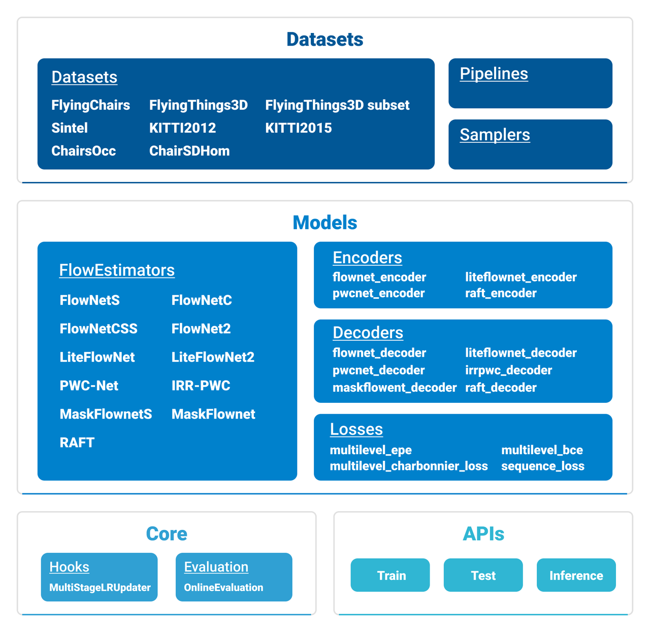
MMFlow consists of 4 main parts, datasets, models, core and apis.
datasetsis for datasets loading and data augmentation. In this part, we support various datasets for supervised optical flow algorithms, useful data augmentation transforms inpipelinesfor pre-processing image pairs and flow data (including its auxiliary data), and samplers for data loading insamplers.modelsis the most vital part containing models of learning-based optical flow. As you can see, we implement each model as a flow estimator and decompose it into two components encoder and decoder. The loss functions for flow models training are in this module as well.coreprovides evaluation tools and customized hooks for model training.apis, provides high-level APIs for models training, testing, and inference,
How to Use this Guide
Here is a detailed step-by-step guide to learn more about MMFlow:
For installation instructions, please see install.
get_started is for the basic usage of MMFlow.
Refer to the below tutorials to dive deeper:
References
Michael Black, Optical flow: The “good parts” version, Machine Learning Summer School (MLSS), Tübiungen, 2013.
Black M J. Robust incremental optical flow[D]. Yale University, 1992.
Butler D J, Wulff J, Stanley G B, et al. A naturalistic open source movie for optical flow evaluation[C]//European conference on computer vision. Springer, Berlin, Heidelberg, 2012: 611-625.
Wulff J, Butler D J, Stanley G B, et al. Lessons and insights from creating a synthetic optical flow benchmark[C]//European Conference on Computer Vision. Springer, Berlin, Heidelberg, 2012: 168-177.
Horn B, Klaus B, Horn P. Robot vision[M]. MIT Press, 1986.
Sun D, Yang X, Liu M Y, et al. Pwc-net: Cnns for optical flow using pyramid, warping, and cost volume[C]//Proceedings of the IEEE conference on computer vision and pattern recognition. 2018: 8934-8943.
Geiger A, Lenz P, Urtasun R. Are we ready for autonomous driving? the kitti vision benchmark suite[C]//2012 IEEE conference on computer vision and pattern recognition. IEEE, 2012: 3354-3361.
Menze M, Heipke C, Geiger A. Object scene flow[J]. ISPRS Journal of Photogrammetry and Remote Sensing, 2018, 140: 60-76.
Menze M, Heipke C, Geiger A. Joint 3d estimation of vehicles and scene flow[J]. ISPRS annals of the photogrammetry, remote sensing and spatial information sciences, 2015, 2: 427.